Tutorial with APOGEE DR10 Spectra¶

Data-Munging¶

Before the data can be run through The Cannon, it must be prepared according to the specifications laid out in the “Requirements for Input” section. One of the requirements is for data to be normalized in a SNR-independent way. TheCannon package does have built-in options for performing the normalization, and we illustrate that here.

For your own project, you would write your own code to read in the data. For this tutorial, we provide the module apogee.py so that you don’t have to figure out how to access all of the relevant information from the .fits files.

First, import the necessary Python packages:

>>> import numpy as np
>>> import matplotlib.pyplot as plt

Now, get the data:

>>> from TheCannon import apogee
>>> tr_ID, wl, tr_flux, tr_ivar = apogee.load_spectra("example_DR10/Data")
>>> tr_label = apogee.load_labels("example_DR10/reference_labels.csv")

Print each of the arrays to inspect the contents. tr_ID is an array of IDs (unique identifiers) for all of the stars. wl is the array of wavelength values. tr_flux is the 2-D array of flux values (spectra for all the objects). tr_ivar is the inverse variances corresponding to tr_flux. tr_label has all of the reference labels for the training step.

Check to make sure that there are 548 spectra with 8575 pixels each, and 3 labels:

>>> print(tr_ID.shape)
>>> print(wl.shape)
>>> print(tr_flux.shape)
>>> print(tr_label.shape)

Now, plot the spectrum for the object with ID ‘2M21332216-0048247’:

>>> index = np.where(tr_ID=='2M21332216-0048247')[0][0]
>>> flux = tr_flux[index]
>>> plt.plot(wl, flux, c='k')
>>> plt.show()

Clearly, some of the pixels have bad values: the flux is 0. Those should have zero inverse variances. Let’s plot the spectrum only with pixels that are good (that is, inverse variance > 0):

>>> ivar = tr_ivar[index]
>>> choose = ivar > 0
>>> plt.plot(wl[choose], flux[choose], c='k')
>>> plt.show()

That’s better. (Note that the spectrum is flat because APOGEE spectra are already continuum normalized.)

To keep things simple in this exercise, we’re going to fit a model using the training objects and then use that model to re-determine the labels for those very same objects. That is, our test objects are identical to our training objects. In practice, you would almost never do this – your test set would be different from your training set.

>>> test_ID = tr_ID
>>> test_flux = tr_flux
>>> test_ivar = tr_ivar

Now that we have all six numpy arrays that we need, we initialize a Dataset object:

>>> from TheCannon import dataset
>>> ds = dataset.Dataset(wl, tr_ID, tr_flux, tr_ivar, tr_label, test_ID, test_flux, test_ivar)

You can access the arrays through this object:

>>> print(ds.tr_ID)
>>> print(ds.tr_flux)
>>> print(ds.wl)

and so on.

Next: TheCannon has a number of optional diagnostic plots built-in, to help the user visualize the results. Some of these plots require knowing the names of the labels. If the user wants to produce these diagnostic plots, the label names must be specified (LaTeX format works):

>>> ds.set_label_names(['T_{eff}', '\log g', '[Fe/H]'])

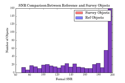
At this stage, two diagnotic plots can already be produced, one with the distribution of SNR in the training and test set (they will be identical in this case) and the other using triangle.py to plot the training label values against each other.

>>> fig = ds.diagnostics_SNR()

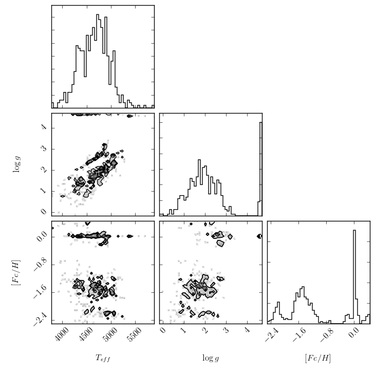
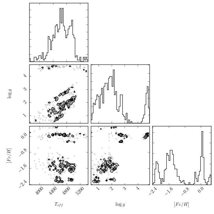
We can also plot the reference labels against each other, to understand the phase space we are dealing with. This plot shows both the distribution of each individual label, as well as its correlations with other labels.

>>> fig = ds.diagnostics_ref_labels()

Next, we normalize the spectra (APOGEE spectra are continuum normalized but not quite in the way The Cannon needs them to be. What you do at this stage will depend on your own unique dataset.)

First, continuum pixels are identified from a pseudo-continuum normalized version of the training set spectra. Pseudo-continuum normalization is performed using a running quantile. In this case, the window size for calculating the median is set to 50 Angstroms and the quantile level is set to 90%. APOGEE spectra come in three chunks, and we want to perform continuum normalization for each chunk separately. For TheCannon to treat spectra in chunks, the ranges attribute must be set:

>>> ds.ranges = [[371,3192], [3697,5997], [6461,8255]]

Even if a spectral dataset do not consist of chunks separated by gaps, one can imagine other reasons for wanting to treat a spectrum as though it had gaps: for example, if different regions of a spectrum behave very differently, it might be sensible to treat each of them separately in continuum normalization. The user should make sure to examine the results of continuum normalization, for example plotting fifty sample continuum fits and continuum normalized spectra.

Pseudo continuum normalization can then be performed as follows:

>>> pseudo_tr_flux, pseudo_tr_ivar = ds.continuum_normalize_training_q(q=0.90, delta_lambda=50)

This can take a while. Once the pseudo continuum has been calculated, a continuum mask is created: True values correspond to pixels that are continuum, False to those that are not. “True” continuum pixels are identified using a median and variance flux cut across the training objects: in other words, continuum pixels are those that consistently have values close to 1 in all of the training spectra. The user specifies what fraction of pixels to identify as continuum, and the flux and variance cuts are determined appropriately. If the ds.ranges attribute is set, then continuum pixels are identified separately for each region (in this case, three regions). This enables the user to control how evenly spread the pixels are.

In this case, we choose 7% of the pixels in the spectrum as continuum, but the best value should be determined through experimentation.

>>> contmask = ds.make_contmask(pseudo_tr_flux, pseudo_tr_ivar, frac=0.07)

At this stage, the user should plot spectra overlaid with the identified continuum pixels to ensure that they look reasonable and that they roughly evenly cover the spectrum. Large gaps in continuum pixels could result in poor continuum normalization in those regions. If the continuum pixels do not look evenly sampled enough, the range can be changed and the process repeated. For this example, we change it as follows:

>>> ds.ranges = [[371,3192], [3697,5500], [5500,5997], [6461,8255]]
>>> contmask = ds.make_contmask(pseudo_tr_flux, pseudo_tr_ivar, frac=0.07)

Once a satisfactory set of continuum pixels has been identified, the dataset’s continuum mask attribute is set as follows:

>>> ds.set_continuum(contmask)

Once the dataset has a continuum mask, the continuum is fit for using either a sinusoid or chebyshev function. In this case, we use a sinusoid; the user can specify the desired order. Again, this is 3 for this simple illustration, but should be determined through experimentation.

>>> cont = ds.fit_continuum(3, "sinusoid")

Once a satisfactory continuum has been fit, the normalized training and test spectra can be calculated:

>>> norm_tr_flux, norm_tr_ivar, norm_test_flux, norm_test_ivar = ds.continuum_normalize(cont)

You can plot a normalized spectrum as follows:

>>> plt.plot(wl, norm_tr_flux[10,:])

Take a look at a few of them. If these normalized spectra look acceptable, then they can replace the non-normalized spectra:

>>> ds.tr_flux = norm_tr_flux
>>> ds.tr_ivar = norm_tr_ivar
>>> ds.test_flux = norm_test_flux
>>> ds.test_ivar = norm_test_ivar

Now, the data munging is over and we’re ready to run TheCannon! Note that the steps above all depend on your particular dataset, and your particular science goals. The steps below are the real core of TheCannon.

Running The Cannon¶

For the training step (fitting for the spectral model) all the user needs to specify is the desired polynomial order of the spectral model. In this case, we use a quadratic model: order = 2

>>> from TheCannon import model
>>> md = model.CannonModel(2, useErrors=False)
>>> md.fit(ds)

At this stage, more optional diagnostic plots can be produced to examine the spectral model:

>>> md.diagnostics_contpix(ds)
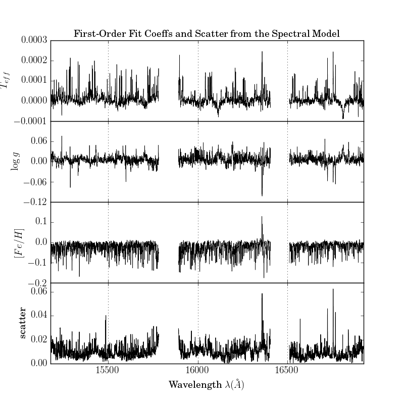
>>> md.diagnostics_leading_coeffs(ds)
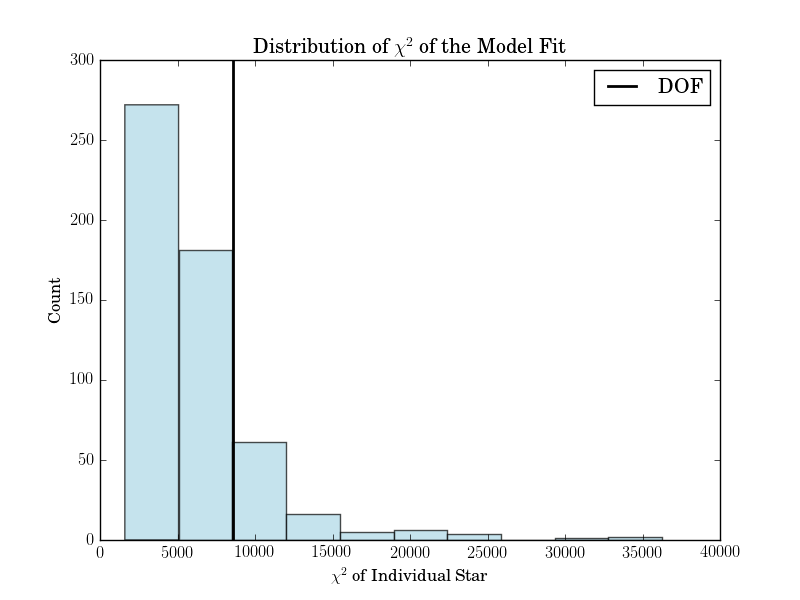
>>> md.diagnostics_plot_chisq(ds)

The first is a series of plots showing the full baseline (first-order) model spectrum with continuum pixels overplotted.

The second is a plot of the leading coefficients and scatter of the model as a function of wavelength

The third is a histogram of the reduced chi squareds of the model fit.

If the model fitting worked, then we can proceed to the test step. This command automatically updates the dataset with the fitted-for test labels, and returns the corresponding covariance matrix.

>>> label_errs = md.infer_labels(ds)

You can access the new labels as follows:

>>> test_labels = ds.test_label_vals

A set of diagnostic output:

>>> ds.diagnostics_test_step_flagstars()
>>> ds.diagnostics_survey_labels()

The first generates one text file for each label, called flagged_stars.txt. The second generates a triangle plot of the survey (Cannon) labels, shown below.

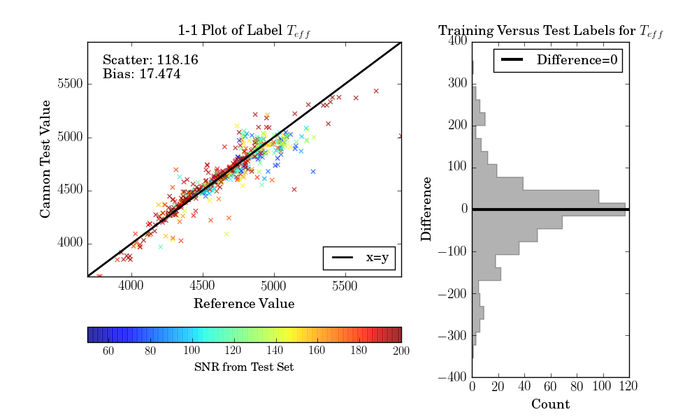
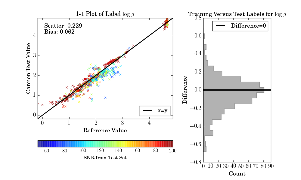
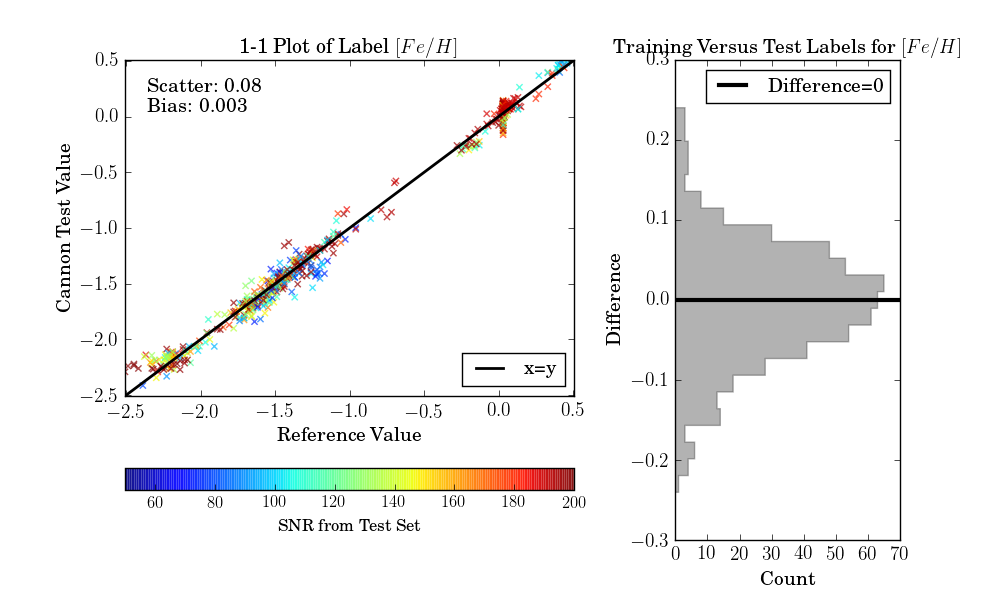
If the test set is simply equivalent to the training set, as in this example, then one final diagnostic plot can be produced:

>>> ds.diagnostics_1to1()